From snapshot to physics
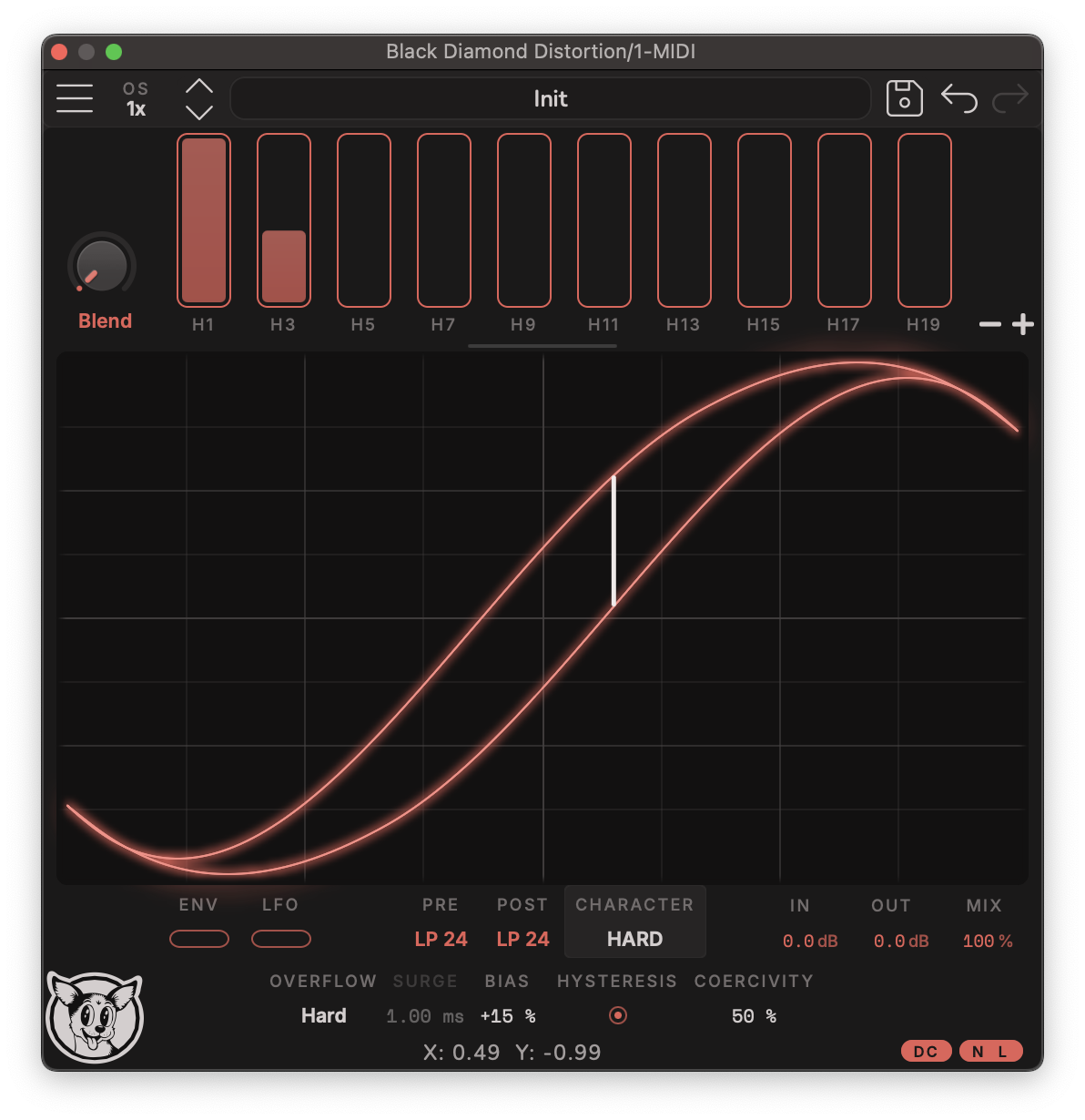
Your drawn curve is a snapshot; the Character panel gives it physics. One panel, five controls: OVERFLOW, SURGE, BIAS, HYSTERESIS, and COERCIVITY.
Hysteresis
The Hysteresis toggle enables a physics-based simulation using the same math that models the magnetic behavior of tape and transformers (a Jiles-Atherton hysteresis model). You might recognize this algorithm’s character from popular tape emulators like ChowTape - the difference is that where ChowTape wraps the hysteresis around an equation specific to real magnets (The Langevin), here it wraps around any transfer function curve you draw. The Langevin is the static part of the magnetic saturation, so the dynamic part is still based on physics but it uses your static transfer function as the building block. The sound now depends on where the signal has been, not just where it is.
Coercivity
Coercivity is the parameter in the physics model that determines how wide the hysteresis loop opens. Low settings add subtle magnetic glue; high settings smear into saturated memory.
A tape-machine footnote: real tape decks add a high-frequency bias signal to control the hysteresis - which is very different from the DC bias below. If you want to emulate high-frequency bias, lower the coercivity.
Bias
BIAS is a DC bias that shifts the signal’s operating point off-center for asymmetric distortion - even harmonics, a different flavor. When you add bias, a dot appears on the curve marking the operating point: drag it to dial the bias in, or double-click to reset it to 0.
Two field notes from measuring analog gear: most of it carries some bias - and the most common “dynamic” behavior isn’t hysteresis, it’s bias that shifts with the envelope of the input. Slam the input and you get more even harmonics; push gently and you get more odd. You can emulate this by mapping the envelope follower to BIAS - see Modulation.
When BIAS is in play you’ll probably want DC blocking enabled (see Gain Staging & DC Blocking).
Overflow and clipping modes
The curve maps input to output up to 0 dB - past that, the signal overflows the transfer function. The 64-bit internals don’t actually overflow; the curve just ends at 0 dB. If that feels limiting, gain staging is the answer: dropping your input gain by 6 dB is essentially the same as having a curve that extends to +6 dB (and likewise for 12, 24, 36…). The payoff for this design is the plugin’s small footprint in CPU, memory, and latency.
As audio passes through, the visualizer highlights the curve up to where your input is hitting. If you don’t want overflow, adjust the gain so the highlight stays inside the curve. Or drive past the boundary on purpose - this is a distortion plugin, after all - and pick an overflow mode:
- HClip (default) - hard-clamps the signal at the boundary.
- SClip - adds a subtle knee at the boundary, which can reduce aliasing.
- Linear - extrapolates the curve along its slope at the boundary; the least aliasing of all modes.
- Mirror - folds the wave back, following the reversed shape of the curve.
- Surge - overshoots clamp gradually over time (below).
Surge
Surge mimics something seen in real analog gear: the signal overshoots, and the circuit takes time to clamp it back down - like a slow diode. The surge dial sets how long the clamp takes. Time-varying distortion from a single knob.